LLS #6: Evaluating Lens Design

When designing a lens or choosing a lens, it's important to know if the lens is good enough for your application. Having a suite of analysis types is an important part of this process. In this post we will cover five analysis types that can be used to evaluate lens performance.

Ray Tracing

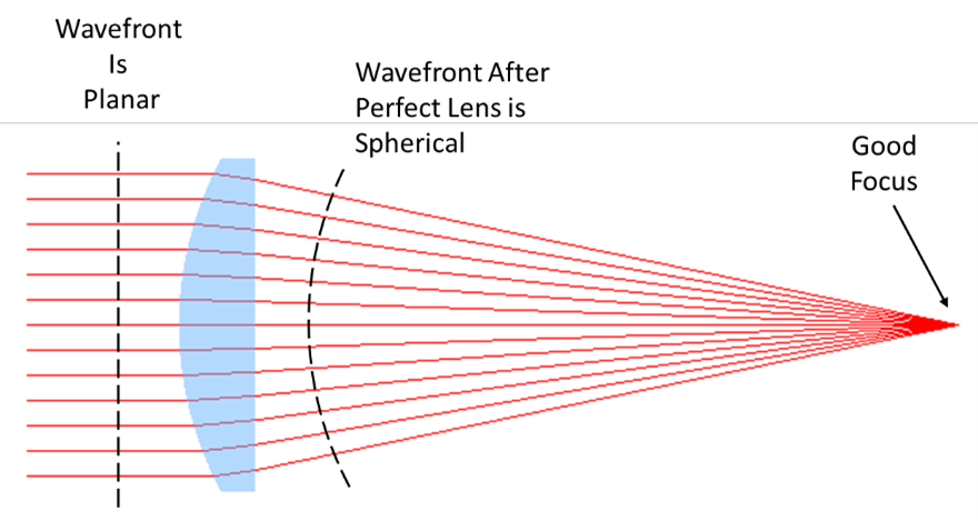
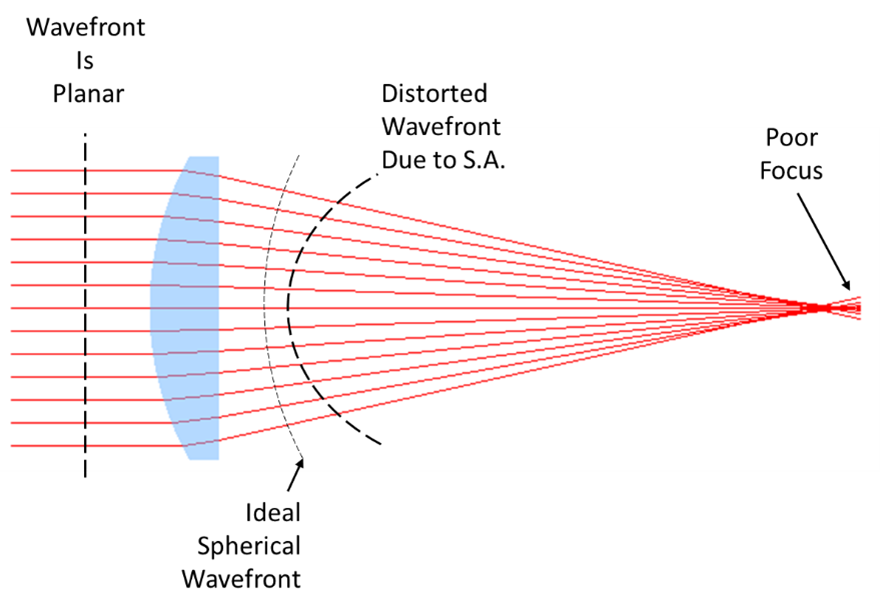
Arguably one of the simplest forms of performance analysis is done by looking at the ray trace through a lens. It can reveal, in rather crude terms, if the lens is focusing the rays to a point (assuming we are evaluating a simple focusing lens). Figure 1 shows ray traces for two short focal length lenses. Figure 1a shows a simple plano convex lens and Figure 1b shows this same lens but with aspheric terms to correct spherical aberrations. Note how the rays in 1a fail to converge to a single point, but the rays in 1b do.

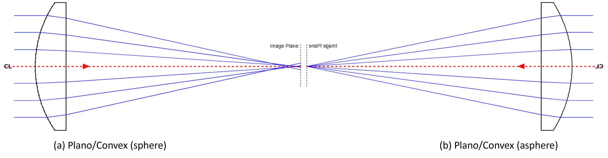
Looking at how rays focus in a plot on a computer screen is judging a lens at the macro level. It’s a good starting point but not sufficient when designing a high-quality lens for a precision laser application.

Transverse Spherical Aberration

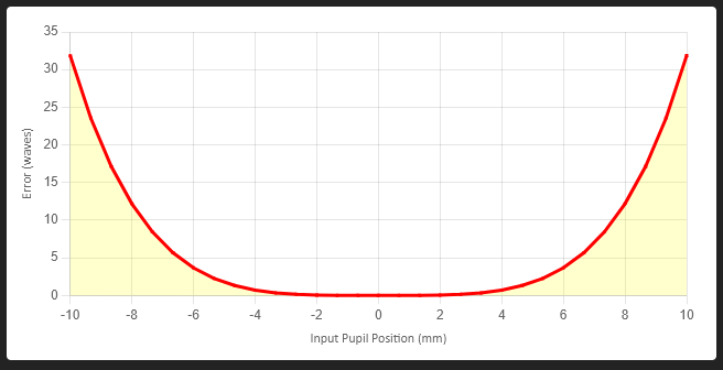
A better way to analyze a lens is by plotting the ray intercept point versus the input ray height. Figure 2 shows a transverse spherical aberration plot for our example lens in Figure 1a.

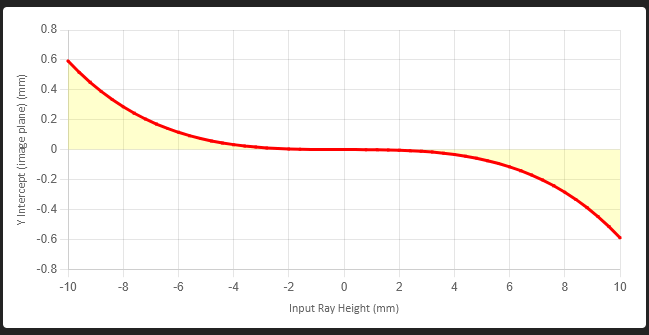
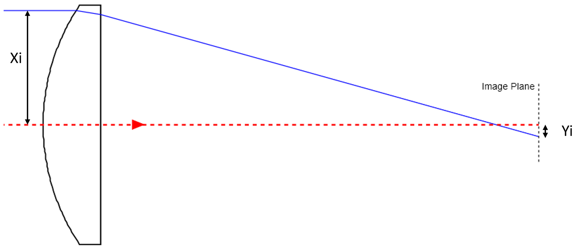
Data for Figure 2 is generated by mapping a set of rays through the center of the lens. The X axis is the input ray height at the lens. The Y axis is the ray height at the image plane (see Figure 3). By tracing a small set of rays through the lens, a transverse spherical aberration plot can be generated rather quickly.

Now we are looking at the lens performance in slightly more detail than ray tracing. As can be seen from plot in Figure 2, the edge ray intercept (10 mm) strikes the image plane at -0.6 mm. The minus sign indicates that the ray strikes the image plane below the central axis. Also note that rays starting at ±3 mm strike the image plane close to zero. But for input heights greater than this, the deviation at the image plane increases exponentially.

A perfect lens would produce a horizontal line at zero on the y-axis. Small amounts of deviation are ok, however, but ±0.6 mm is definitely NOT ok. As a very rough rule of thumb, the maximum spherical aberration should be less than about 1 wavelength, which in this case is 1.07 μm, if we require the best possible lens.

Spot Diagram

The spherical aberration plot traces a small set of rays in one plane only, the Y-axis in this case. We can trace rays through the full aperture of the lens and then plot their (x,y) rays position at the image plane. Figure 4b shows a spot diagram plot for our example lens. Figure 4a shows the ray positions at the entrance to the lens. Usually we don't bother plotting the spot diagram at the lens, only at the image plane.

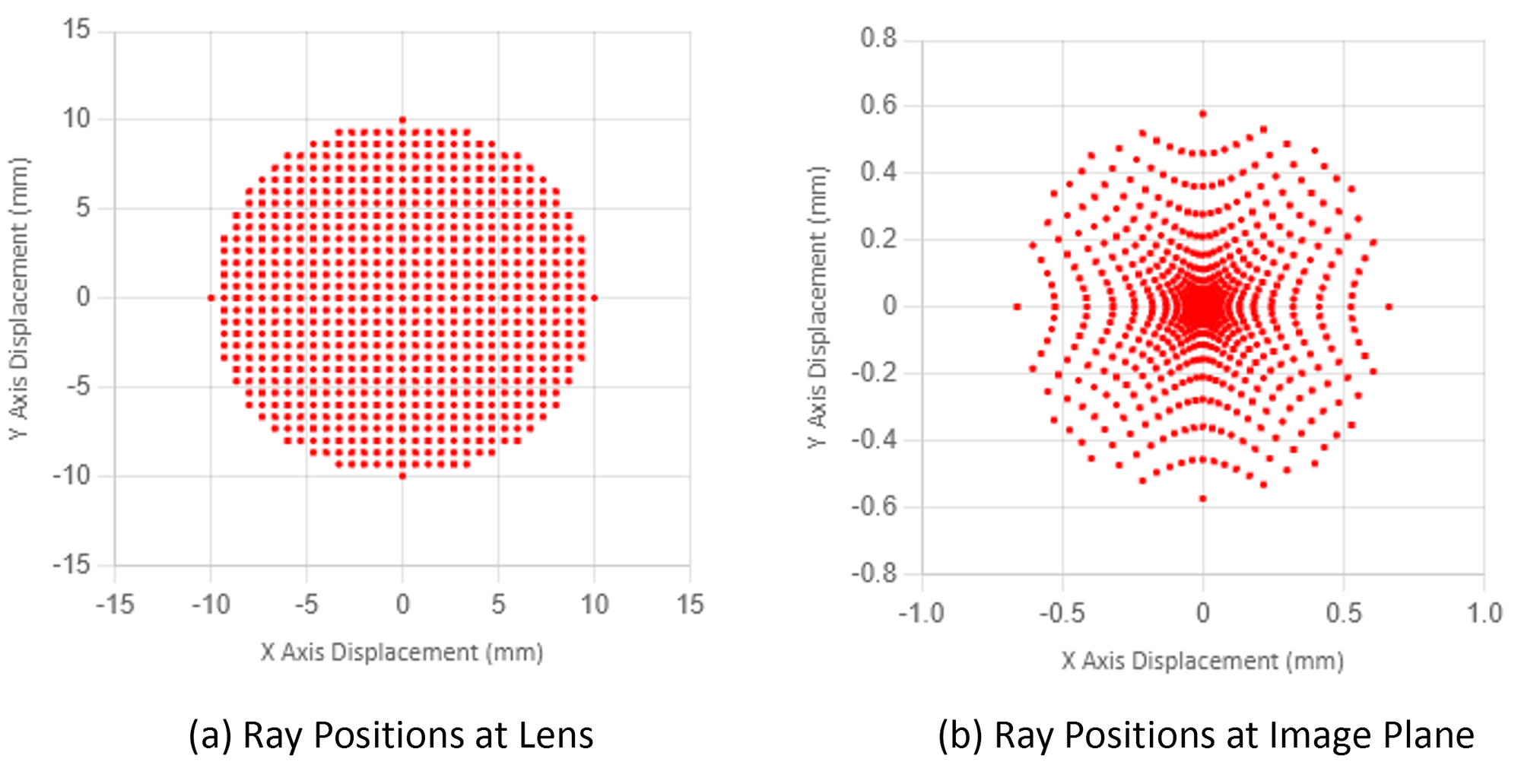
We can use the same rule of thumb for this plot as the transverse spherical aberration plot. Ideally we want spot diagram where all rays fall within one wavelength diameter when designing a precision lens. "Precision lens" in this case just means a lens that will focus the spot to the smallest possible diameter.

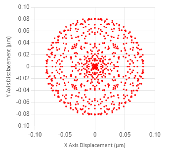
Figure 5 is a spot diagram plot for the aspheric version of this lens (Figure 1b). Note that the X and Y axis scale is now in microns. In this lens spherical aberrations have been minimized (< 1/10 of a wavelength).

Spot diagram plots provide a lot of information of rays at the image. Since the full aperture is traced it is most useful for lenses that are used off-axis.

Wavefront Error Plot (cross section)

Spherical aberration plots and spot diagrams are generated by geometrical tracing ray vectors through a lens using simple trigonometry and Snell's Law. Another analysis types is wavefront error. For this analysis, we assume that the incoming light or laser beam wavefront is planar at the entrance to a lens. Ideally the lens converts this planar wavefront to a spherical wavefront.

If we want all rays to focus to a common point at the image plane, the rays must have a spherical wavefront. But at the focus, the wavefront is planar before the beam diverges again. In the real world, lenses convert a planar wavefront to a spherical wavefront with some amount of deviation from a sphere.

Wavefront error plots are the calculated wavefront deviation from the ideal wavefront, be it planar or spherical. Figure 8 is the wavefront error plot for the lens in Figure 1a.

Wavefront error plots are typically in waves (sometimes just λ)at the design wavelength, in this case 1.07 μm. A wavefront error of ~32 λ is very bad for almost all optical applications. A good rule of thumb for precision lenses is probably <1/10 λ, although <1/20 λ is better if we are striving for the best possible design.

In the optics field, one will often hear a wavefront error rule of thumb to be <1/4 λ. This rule was adopted for vision systems decades ago and it is still widely used today. And it seems to have been adopted into the laser industry also. However, for precision optics for laser applications, this rule is not sufficient to get the smallest possible focused spot.

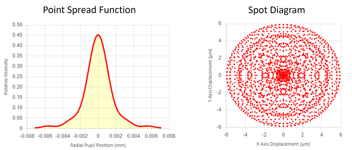
Point Spread Function

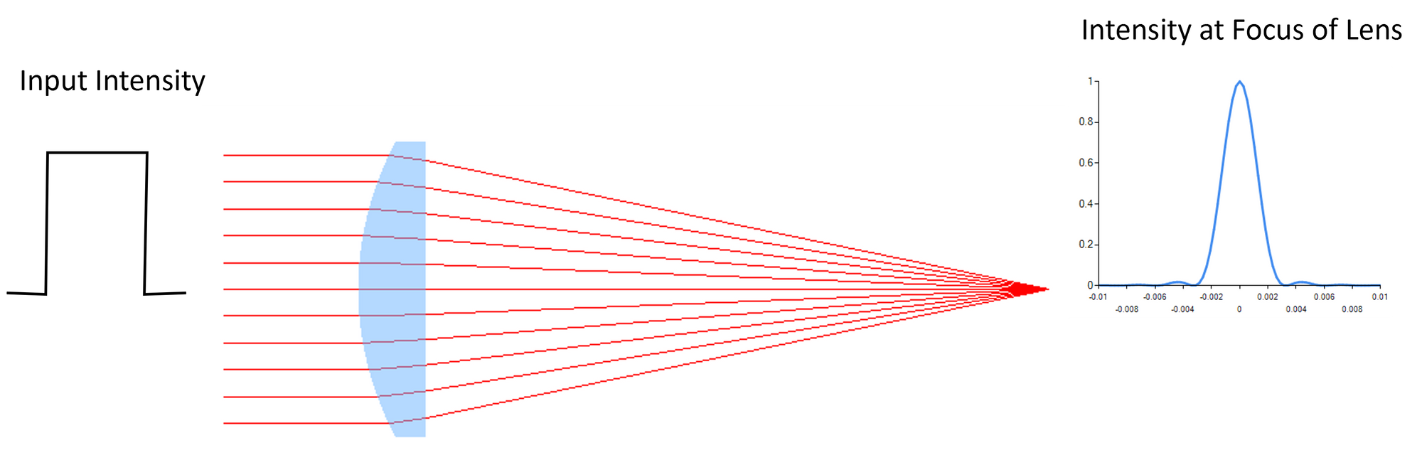
The Point Spread Function (PSF) is yet another way to evaluate a lens. Almost all the analyses so far have relied of geometric optics and geometric ray tracing techniques. PSF analysis is a diffraction based analysis that uses discrete Fourier Analysis.

PSF analysis is a very good way to determine the focusing quality of a lens. This analysis assumes that the input beam comes from a point source (hence the PSF name) very far from the lens – which means that the beam is essentially collimated when it enters the lens. It also means that the intensity distribution of the input beam is flat or uniform across the clear aperture.

The lens will transform this flat top collimated beam to a focused beam with an airy disc distribution if the lens is aberration free.

The size of the airy disc in the focal plane, again assuming a perfect lens or aberration free lens, is given by:

Here,

D_airy is the diameter of the focused beam measured at the first minimum,

λ is the wavelength of light,

f is the focal length of the lens, and

D_Input is the diameter of the input beam - assuming the energy profile is a flat top.

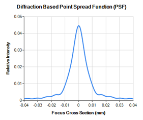
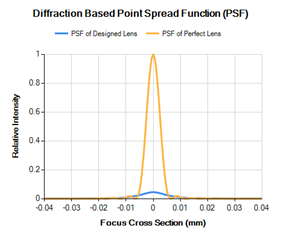
Of course, for a lens that has spherical aberrations the quality of the focused beam is degraded. Below is the PSF analysis of a less than perfect lens. Note that the peak intensity is extremely low (remember perfect lens PSF peak intensity should be 1.0). This loss in energy at the peak means that more of the energy is distributed in the wings of the beam.

We can plot the perfect PSF on the same plot as a one in Figure 11. The degradation of the performance of the real lens is immediately apparent. Perhaps an aspheric lens should be considered in this case if the application requires a precision focus.

In the rare instance that the actual input laser beam is a collimated, coherent, flat top, monochromatic beam, then the PSF plot is a true representation of the focused spot size and shape. If the input beam is some other type, such as gaussian or higher mode beam, then the PSF will only indicate if the lens will focus the beam to it's smallest spot.