LLS #4: Designing Laser Lenses

Designing lenses for a laser application is simplified by the fact that the lens must work at only one wavelength – the wavelength of the laser. This is true for most laser applications, but there are some exceptions which might be discussed in later posts.

Lensmaker's Equation

The basic lens is designed by first picking the desired focal length and then using the Lensmaker’s Equation for thick lenses to design the lens.

In this equation

f is the focal length of the lens,

n is the index of refraction of the lens material,

R1 is the radius of curvature of side 1 of the lens,

R2 is the radius of curvature of side 2 of the lens,

d is the center thickness of the lens.

When starting a lens design, the parameters that we know are the wavelength of the application which will determine the lens material and the focal length (f). We should also have good idea of the beam size and shape.

The laser and application usually dictate the lens material. For example, a high-power fiber laser will probably use a fused silica lens, a pointer laser will use a low cost BK7 lens, and a high-power CO₂  laser will use a ZnSe lens. But for non-high power CO2 lasers other materials like GaAs and Ge lenses (to name two) can be used. The material is important because the lens material and the wavelength of the application will determine the index of refraction (n) in equation 1. So, if the application is a high-power fiber laser at 1.07 μm, then the most likely lens material is fused silica. Fused silica has an index of 1.45 at this wavelength.

It’s also likely that you will know what thickness of lens you require. Thickness of a lens is usually determined by the lens holder limitations, but it can also be influenced by laser power. For example, a high power ZnSe lens should be relatively thick compared to a lower power application because the heat generated by the high power is dissipated by the thicker lens. This is not necessarily true for fused silica in a high-power fiber laser application. So now we have f, n, and d in equation 1.

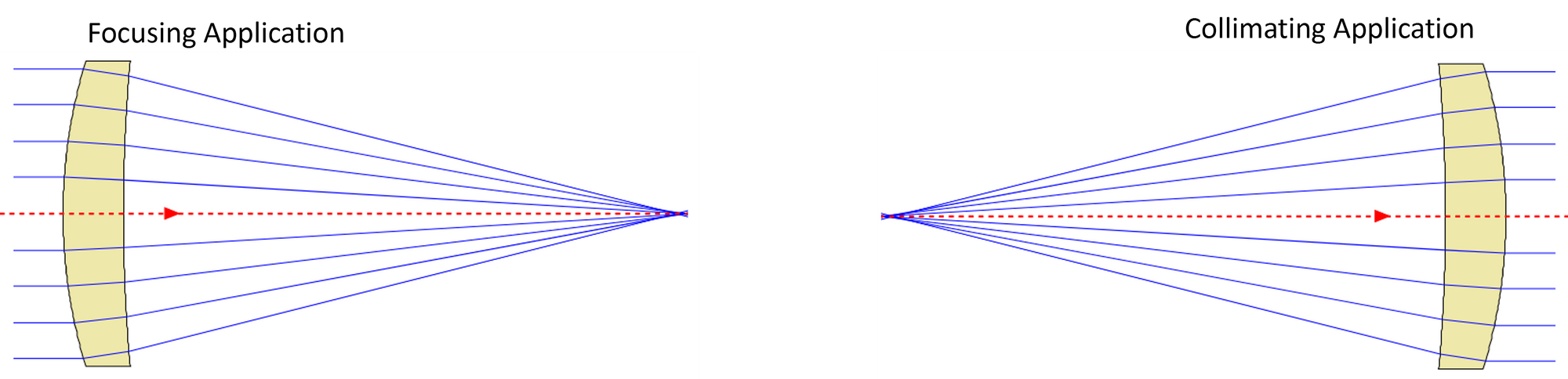
Rule of Thumb: When designing laser lenses it is usually a good idea to make the steepest curved surface face the collimated side of the beam. So if we want to focus a collimated beam, then the steeper curved surface should face that side.

Plano Convex (Po-Cx) or Plano Concave Lenses (Po-Cc)

The next issue is to solve Equation 1 for R₁ and R₂. This is relatively simple if we want a Po-Cx lens. A flat (plano) surface has a radius of curvature of infinity, so in Po-Cx lenses, R₂ is set to infinity (which means 1/R₂  = 0) and we change R₁ to obtain the desired focal length.

Equation 1 simplifies to:

Since we know f and n, solving this equation for R₁ is trivial.

Notice that the center thickness, ‘d’, does not influence the focal length, ‘f’, of a Po-Cx or Po-Cc lens.

Bi-Convex (B-Cx) or Bi-Concave (Bi-Cc) Lenses

A second slightly more involved solution occurs when we want to design Bi-Cx or Bi-Cc lenses where R₁ = -R₂. In this case the solution to Equation 1 is of a quadratic form where one solution is positive, and one solution is negative. We pick the positive solution to the quadratic and then assign it the same sign as the focal length. So, if we want a Bi-Cx lens shape, we make R₁ positive and R₂ negative. For a Bi-Cc lens we make R₁ negative and R₂ as positive.

Best Form Lenses

For a given focal length ‘f’, index ‘n’, and center thickness ‘d’, Equation 1 has an infinite number of solutions for R1 and R2. If we allow R1 and R2 to be any value, then we need some other way to pick radii that will provide us the best lens for our application. We’ll call this type of lens a Best Form lens.

The Best Form lens for an application can be found by considering lens aberrations. Fortunately, in laser applications the primary and usually the only lens aberration is spherical aberration (SA).

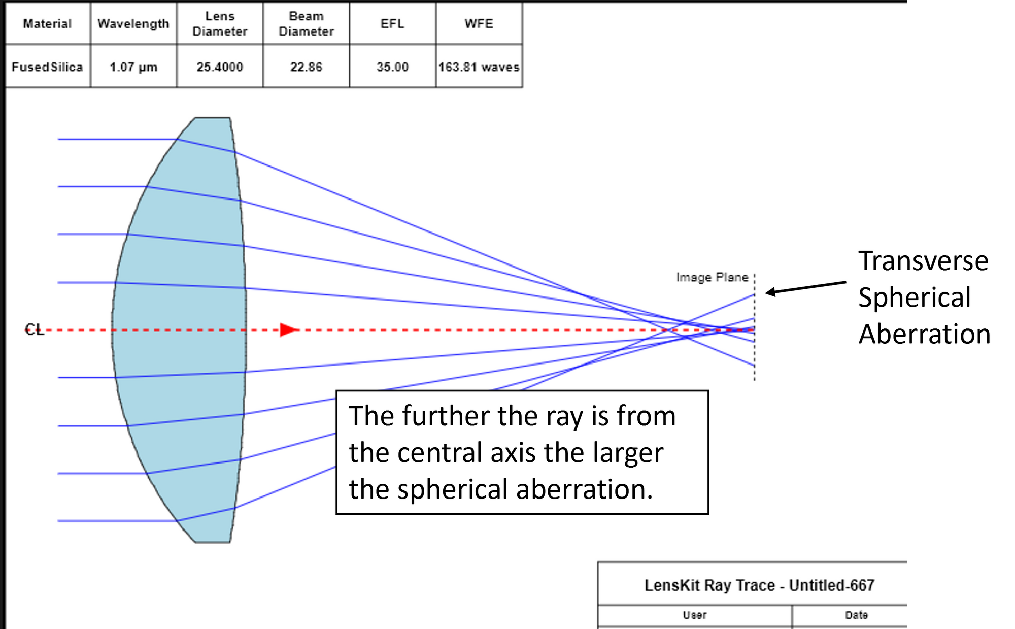
Spherical aberration is simply the deviation of rays at the focal plane based on their distance from the optic axis. One would think that all rays passing through a spherical lens would focus to one point at the image plane. But, in fact, every ray passing through a spherical lens focuses to a slightly different point on the image plane. The amount of lateral deviation at the image plane is called transverse spherical aberration.

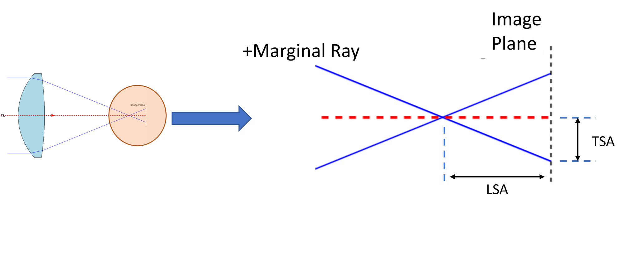
In the lens designer world, spherical aberrations are calculated in one of two ways. Transverse spherical aberration (TSA) is found by calculating the ray height above or below the central axis at the theoretical image plane defined by the focal length of the lens. Longitudinal spherical aberrations (LSA) is defined to be the axial difference between where the ray crosses the central axis and the axial location of the image plane.

In an ideal world we would want all of the rays to come to a common focal point at the image plane. But this does not occur (exactly) with spherical lenses. It is possible, though, to design a Best Form lens that minimizes spherical aberrations. The figure below shows three spherical lenses all of which have a 35 mm focal length. Note the difference in spherical aberration of each lens.

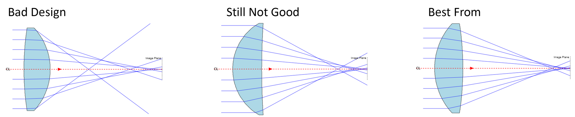
It's obvious from Figure 2 that in order to find the best form lens, we need to minimize spherical aberration. For simple lenses this is done by calculating the deviation of the marginal ray from the axis at the image plane. The marginal ray is just the ray that passes through the lens at the furthest point from the axis.

The marginal ray location (Figure 3) is dictated by the application. If we have a laser beam of 20 mm full diameter (not to be confused with a gaussian diameter), then the marginal ray height (h) will be 10 mm.

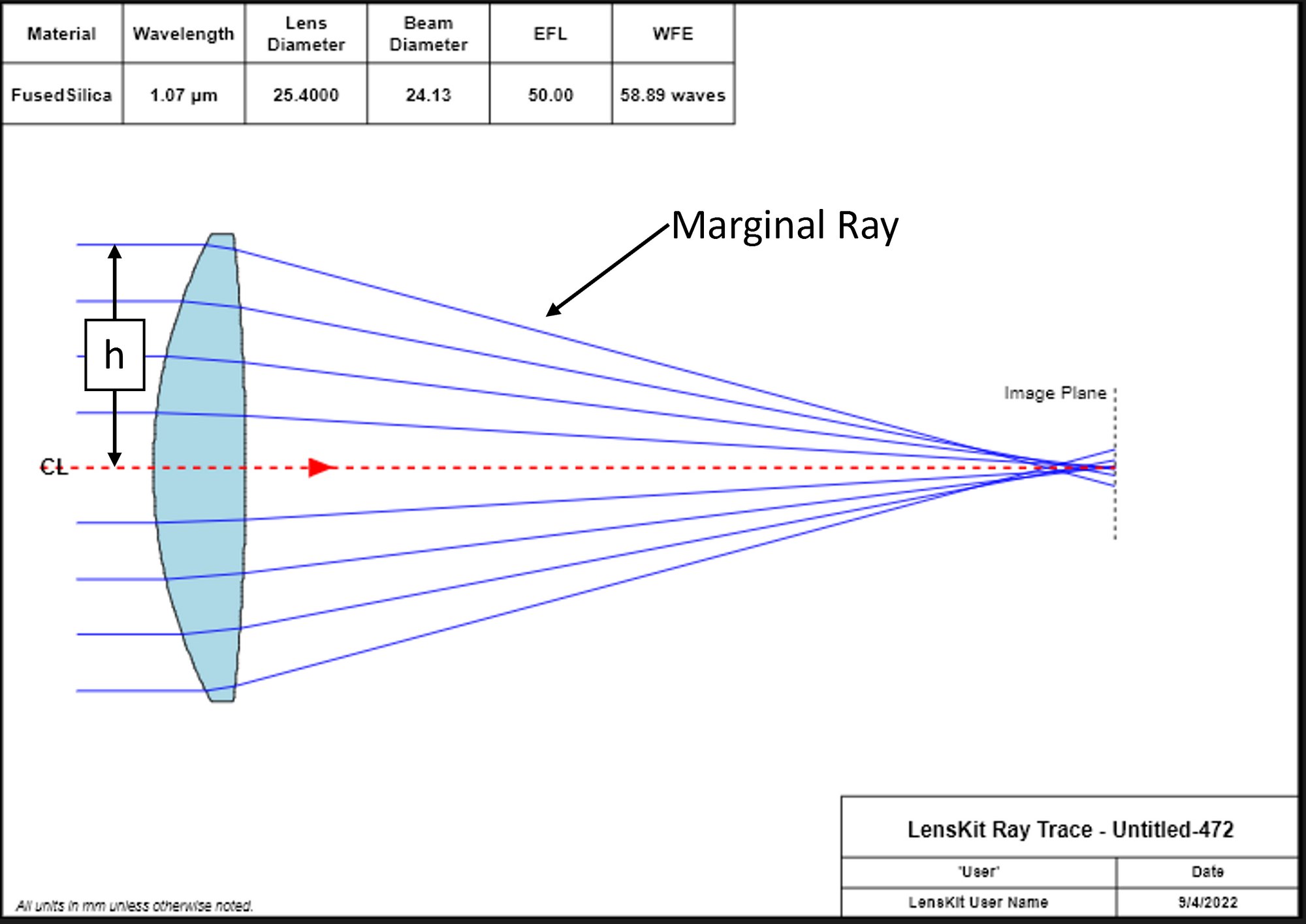
It bears repeating (see Figure 1) that larger beams will have more spherical aberration than smaller beams when passed through the same lens. The key point here is that when we design or choose a lens to use in our application, it is important to know the laser beam parameters.

Spherical aberrations are easily calculated using a bit of vector math and Snell's Law. But there is a somewhat complicated closed form equation for calculating SA of the marginal ray and finding the best form lens shape. If the reader is interested they should read section 9 of Jenkins and White, "Fundamentals of Optics", with special attention to sections 9.3 to 9.5 and equation 9e. But we will give a short summary of this method here. This work will assume that we are designing a lens that will focus a collimated beam.

First we should define a simplified version of the Lensmaker's Equation (Equation 1). If the lens is thin and the R₁ x R₂ is large, then Equation 1 can be simplified to what is called the "Thin Lens Equation."

Using the thin lens equation it is possible to derive (following Jenkins and White reference) an equation for a ray error, ξ. The property, ξ, does have a direct relationship to longitudinal spherical aberration.

where

As before, f is focal length of lens, and n is the index of refraction of the lens material at the design wavelength. The quantity h is the ray height above the central axis (see Figure 3). Equation 5 introduces two new quantities q (shape factor) and p (position factor). For simple focusing lenses that focus a collimated or almost collimated beam, the position factor, p, reduces to a value of -1. It is unitless. See the end of this post, Going Further - Position Factor P Definition,  for a strict definition of the position factor.

The shape factor is an important part of equation 5 and it is related to the radius of the lens. The shape factor, q, is defined to be:

Once focal length and index are fixed, and we know the maximum ray height from our input laser beam, Equations 5 and 6 can be used to plot the longitudinal spherical aberration (LSA) given any  shape factor, q. The plot below shows this result for the lens shown in Figure 3.

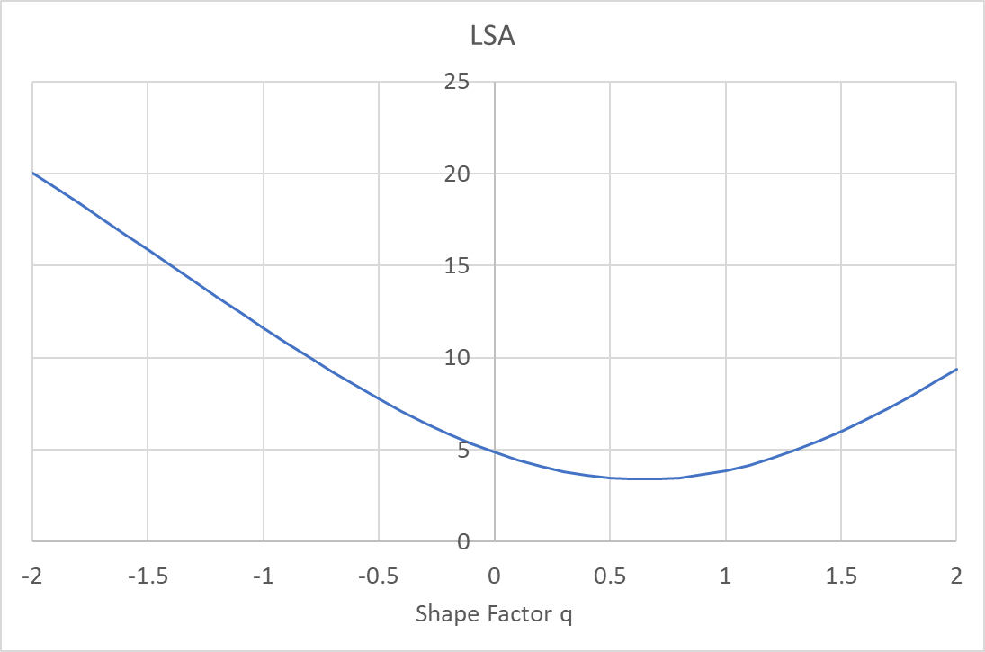
This graph shows that the there is a shape factor value where spherical aberrations are a minimum (q ~ 0.64). It's not necessary to plot Equation 6 for every combination of f, n, and h. We can find the shaper factor where ξ is at a minimum by taking the first derivative of Equation 6 with respect to the shape factor q.

Then the minimum of Equation 8 is found simply by setting dξ/dq = 0 and solving the equation for q. It results in:

Now that we have the best shape factor for a lens, we can calculate the ratio of R₁ to  R₂ by re-arranging Equation 7 into something more useful.

Using this result, the thin lens equation (Equation 4) can be modifying into terms of only one radius and solving for that radius.

So now we have all the tools we need to design a best form lens. Using Equations 9, 11, then 10, we design a best form lens. Using the example in Figure 3, we set f = 50 mm and the index of Fused Silica at 1.07 μm is 1.44966.

First we calculate a q factor from Equation 9:

q = 0.6386

Then calculate R₂ using Equation 11:

R₂ =  -124.43 mm

Then to get a value for R₁ we re-arrange Equation 1:

Using this equation we get:

R₁ = 27.10 mm

The drawing below, Figure 5, is a lens designed by lenskit.app - this is the same design as shown in Figure 3. You will note that R₁ is almost an exact match with our hand calculated estimate above. R₂ is a little bit  different due to the fact that lenskit.app uses the thick lens or Lensmaker's Equation throughout to find the best form lens. Doing so produces a more cumbersome set of equations, but we can get pretty good results using the thin lens equation for estimating R2.

Aspheric Lenses

The ray trace plot in Figure 3 shows a massive amount of spherical aberrations. Although it suited our purposes for explaining how to design a best form lens, it would probably not be useful in the majority of laser applications. Near the top of Figure 3 is a box labeled WFE. This stands for Wave Front Error and it is a measure of how much error there is in the lens. We'll discuss performance metrics in more detail in a later post but suffice it to say that 58.89 waves of WFE is very poor.

Traditionally, when designing a laser lenses with a large spherical or wavefront error, the designers only choice was to 'split' the lens into multiple elements. Doublets were a pretty common way of designing a low aberration lens in these demanding applications.

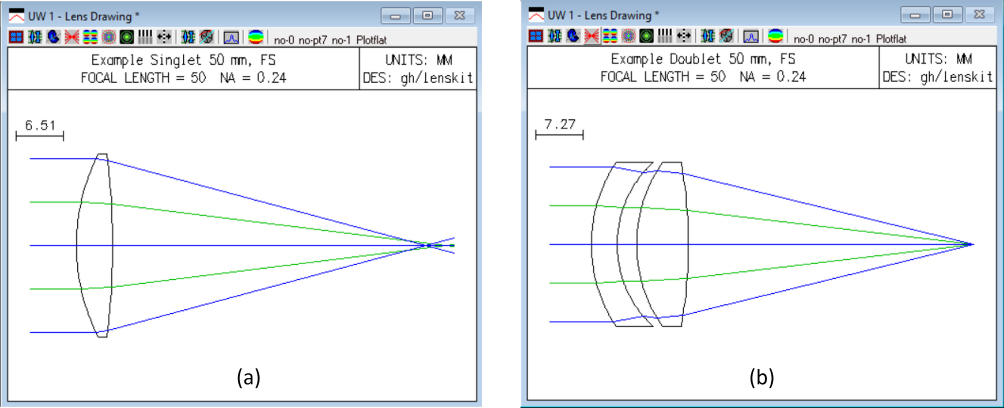
Figure 6 show the design of a 50 mm EFL lens under the same conditions as shown in Figure 3 above but this time designed in the OSLO lens design program. Figure 6a shows the singlet version and Figure 6b shows the doublet version. It's immediately obvious that the rays in (b) converge much better that in (a). The OSLO program reports the wavefront error for (a) is ~50 waves and for (b) it is ~9 waves. A significant reduction.

Designing multi-element lenses with all surfaces being spherical was a pretty common method for improving lens performance until the 1980's. But multi-lens assemblies are expensive, and when used in high power lasers, they can cause severe thermal issues.

Aspherizing a lens is a way to design a lens with zero spherical aberration or zero wavefront error. Well, nothing is perfect, but the aspheric lens can be designed to be very close to it for certain lens designs.

Up Next:

LLS #5: Aspheric Lenses

Under construction.

Lenskit BlogGary Herrit

Going Further - Position Factor P Definition

Following the Jenkins and White, "Fundamentals of Optics", work we have to first define another equation called the lens equation.

Lens Equation

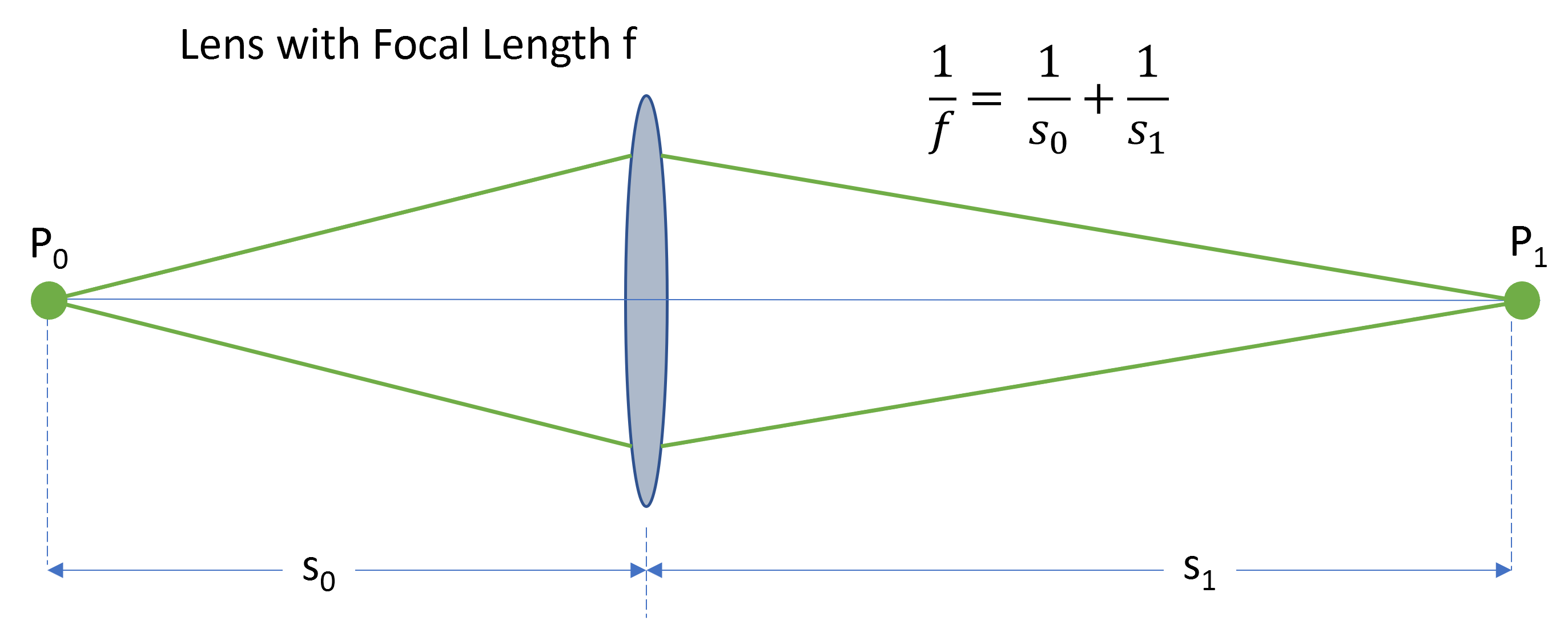
In order to first understand the position factor, we have to introduce a new term - conjugate distances. Conjugate distances, a term found most often in discussing imaging properties of a lens, have a simple relationship:

Here, f is the focal length of the lens, s₀ is the object distance, and s₁ is the image distance. This is usually called the lens equation. The conjugate points P₀ and P₁ and their conjugate distances s₀ and s₁ are shown below.

The Position Factor Defined

If a lens is used in this way then the position factor is given by the following:

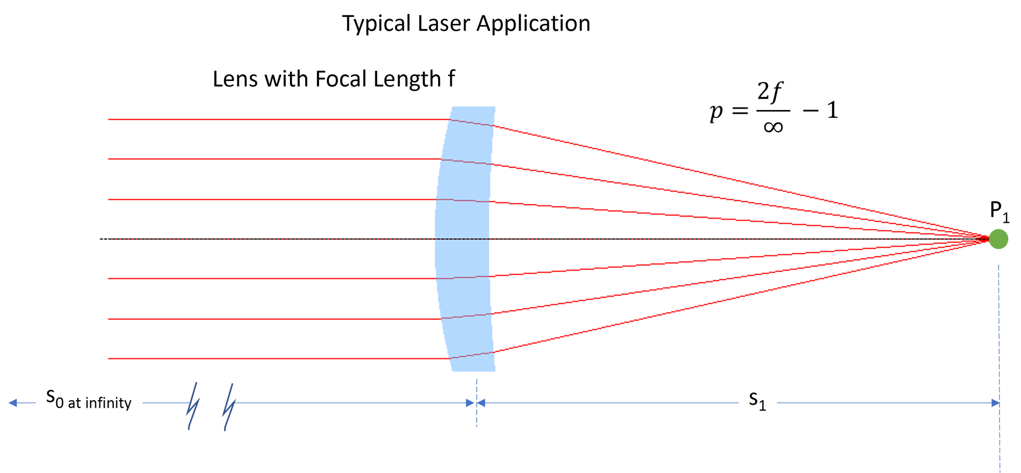
Solving this equation in terms of f and s₀ can be accomplished by solving the thin lens equation for s₀ and using this in the position factor equation. Now the position factor equation has the form:

This factor can be used for the general case of light focused by a lens. But for most laser applications, the incoming beam is collimated like the image below. For collimated light, s₀ is effectively infinity. Under these conditions, p = -1.

This greatly simplifies Equation 5 above.