LLS #5: Aspheric Lenses

In LLS #4: Designing Laser Lenses we found that lenses using only spherical surfaces have some amount of spherical aberration. The magnitude of the spherical aberration can be quite small or quite large depending on focal length, laser beam diameter, lens shape, and index of refraction of the lens material. Adjusting these four parameters can only take you so far in minimizing spherical aberrations, however.

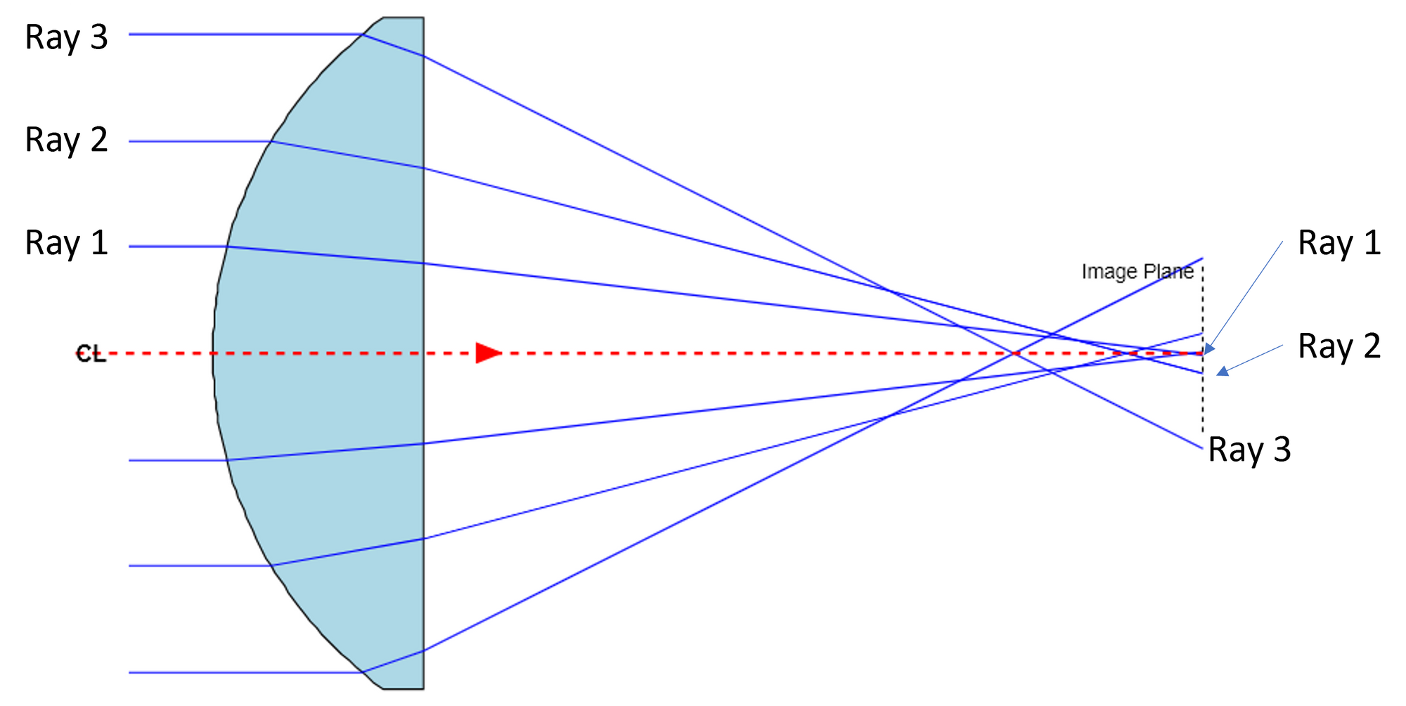
Figure 1 is a ray trace through a basic laser lens with a short focal length. It’s obvious from the ray trace that rays furthest from the center are focused more strongly than rays near the central axis (for example ray 3 versus ray 1).  This is an inherent property of spherical surfaces. Spherical aberrations can be corrected by adjusting the surface curvature such that the surface ‘flattens’ as it gets further from the center.

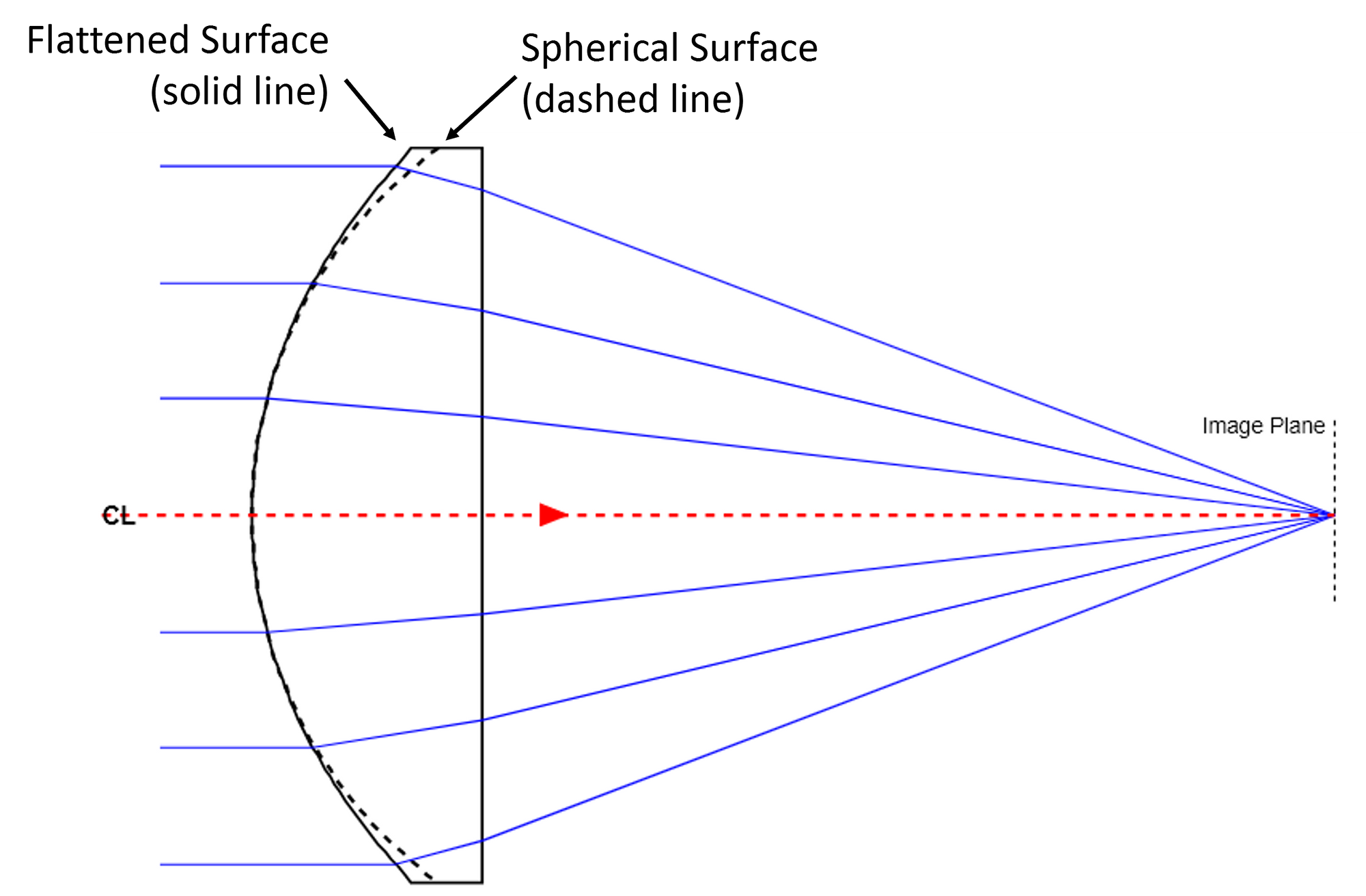
The next figure (Figure 2) shows a comparable lens that has the surface flattened to correct for spherical aberrations. Note that all the rays come to a common focal point at the image plane. In this figure the original spherical surface (dashed line) is superimposed on the flattened surface. As expected, the surface slope at the edge of the optic is smaller than the surface slope of the original spherical surface.

Spheres to Aspheres

Before describing how to aspherization a lens to minimize spherical aberrations, let’s take a step back and discuss in a little more detail spherical lenses. When designing a lens with spherical surfaces, the simple rules as described in LLS #4 are sufficient to get the best design or an application. It is not necessary to resort to more detailed ray tracing to design the lens. Although it must be said that calculating the shape factor (p factor in LLS #4 – Going Further) is a quite simple way of ray tracing the marginal ray through spherical lenses.

If we want to design more complex lenses that use conic sections and aspheric terms, then we need to do detailed ray tracing. This also means that we need to develop an algorithm that will allow us to trace a ray to a lens surface, refract it into the lens and to surface 2, and finally trace the ray to the image plane.

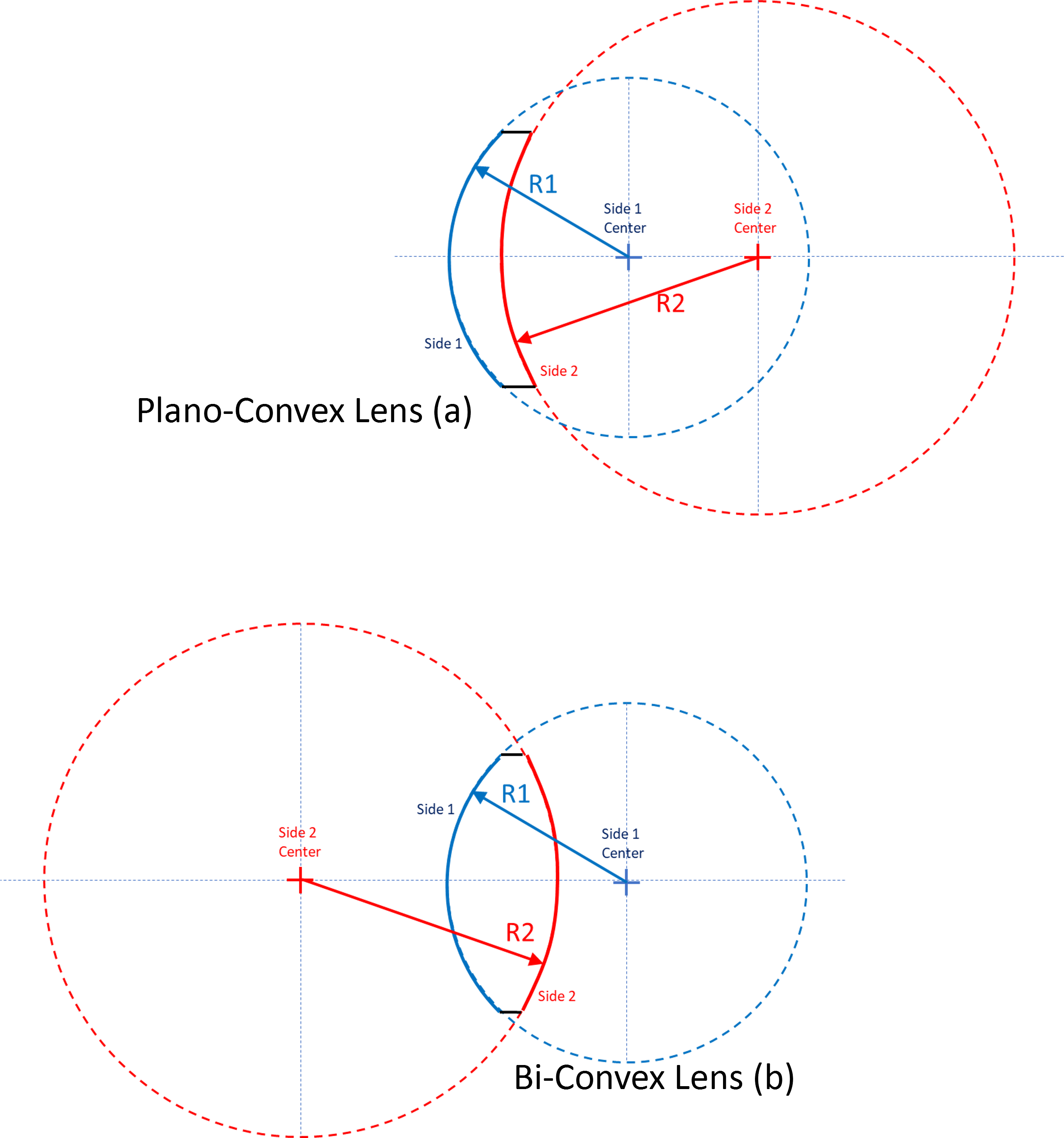
Figure 3 shows two types of lenses that use spherical surfaces. Figure 3a is a positive meniscus lens. Note that the radii for both surfaces are to the right of the lens which makes the radii positive. Figure 3b is a bi-convex lens with side one being a positive radius and side 2 (with center to left of the lens) is a negative radius.

The segment of the circle that is used to construct the lens can be calculated using the standard equation for a circle:

However, ray tracing a light ray through a lens requires knowledge of the position of the lens surface in space and the slope of the surface at the ray intersection point. In order to efficiently calculate these values, we can move the coordinate system to the surface vertex and derive an equation for the surface "sag" which is in the Z-direction.  Figure 4 shows this graphically.

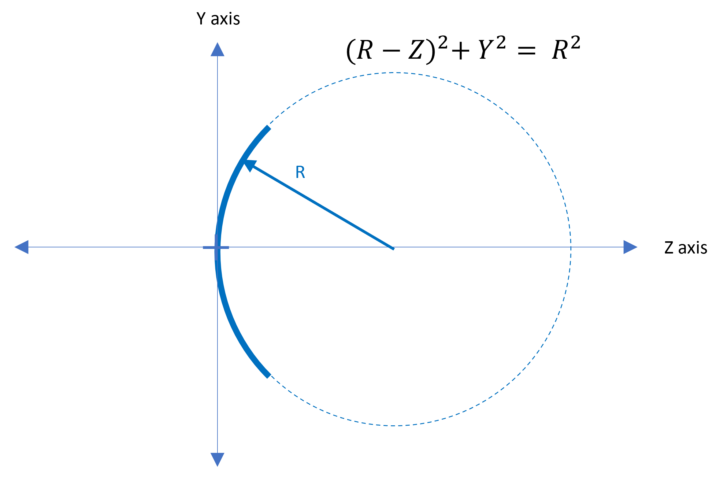
Note also in Figure 4 that we have changed our axes to conform with typical lens design coordinate systems where the Z axis is the propagation axis. Lens design systems usually use a right-hand coordinate system, so the X axis is into the page. The sag is calculated by solving the modified circle equation shown in Figure 4 to solve for Z.

So far we have considered the lens in 2 dimensions only. This is sufficient in some cases to adequately design and optimize simple laser lens which are rotationally symmetric. However, we can add the 3rd dimension to Equation 2 by letting r²= X² + Y² where small r (not to be confused with the surface radius R) is the radial distance from the center of the optic.

Now we have an equation that will define the surface location, Z(r), and the surface slope, dZ/dr.

Conic Sections

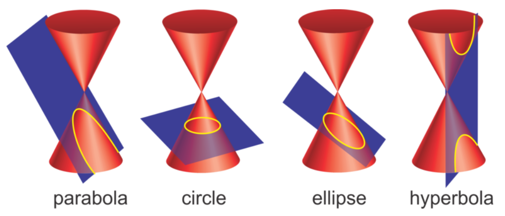
Spherical surfaces produce spherical aberrations in a focused beam. But they are not the only geometric shape that can focus a laser beam. Circles and spheres are, after all, just a special case of an ellipsoid. Conic surfaces are sections of a cone, and they can take on various shapes depending on the angle that the section is take relative to the cone. Figure 5 (https://www.ck12.org/book/ck-12-algebra-ii-with-trigonometry-concepts/section/10.0/) shows the four types of conic sections.

Parabolas and ellipses are widely found in variety of optic applications. Even in simple laser lenses they can be useful in optimizing the lens shape to reduce aberrations. And as it turns out, it is n0t too difficult to solve the general equation of a conic for sag.

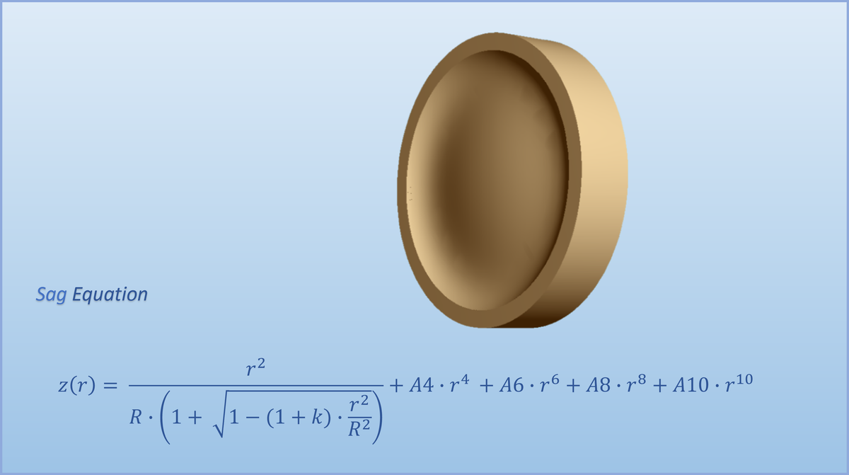
In this equation we added the additional variable k, which is just the conic constant for the surface. Equation 4 is commonly used in lens design programs of all types.

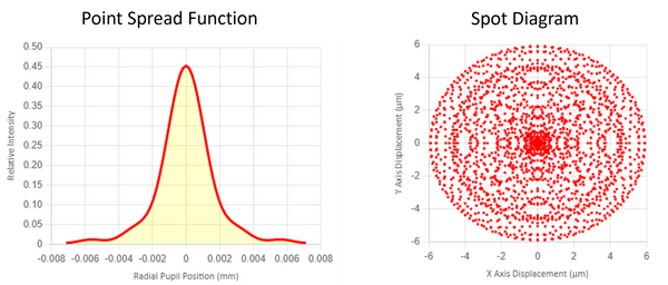
Using the same lens setup of Figure 1 but optimizing it using a conic surface profile the spherical aberrations can be significantly reduces.

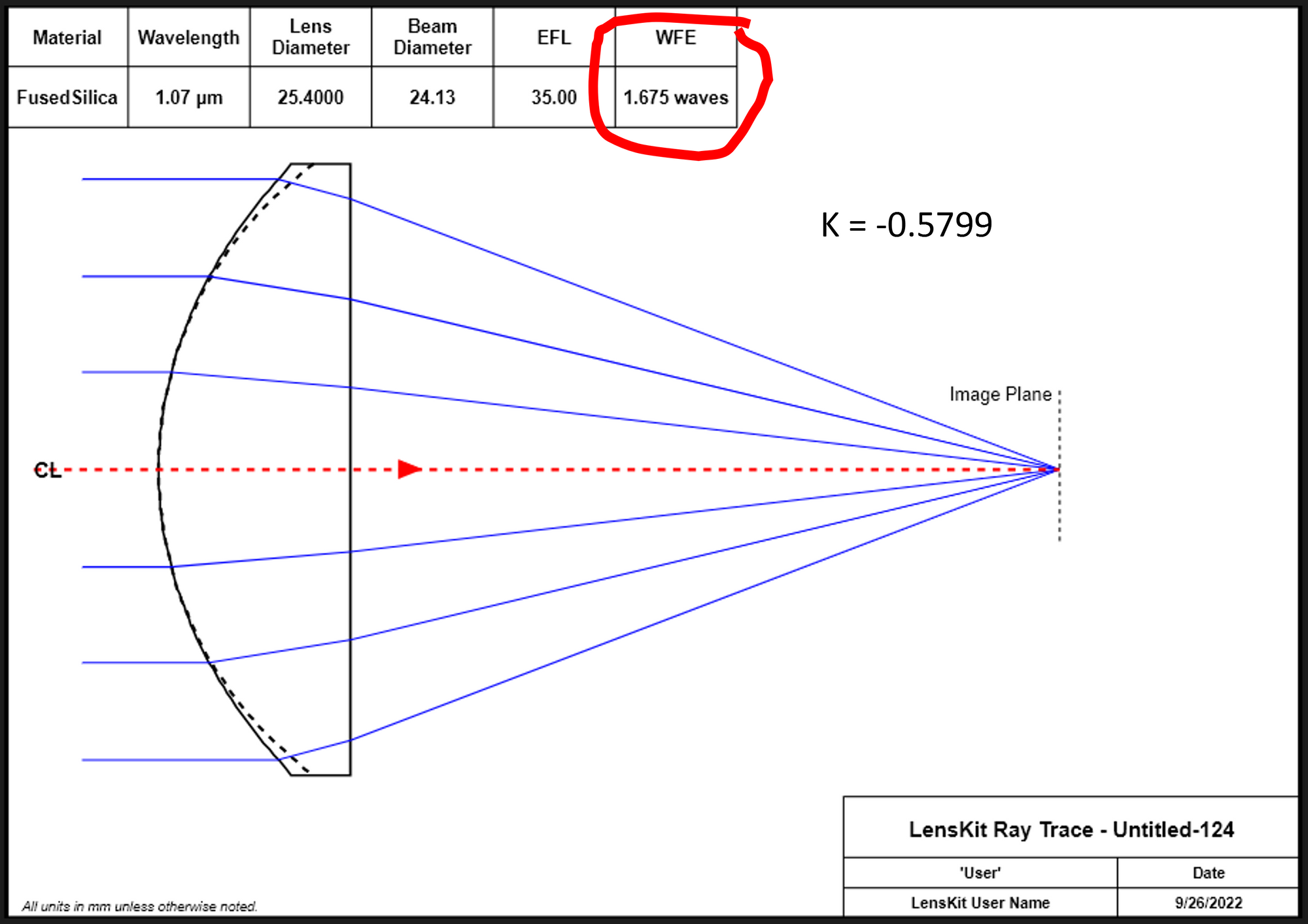
Two things to note are that all the rays appear to focus to the same spot. Although in this graphic it is difficult to see the details. The peak-to-valley spherical aberration magnitude for this conic lens about 0.02 mm. The same P-V spherical aberration magnitude for the spherical lens of Figure 1 is almost 8 mm - a 400x improvement!

Also note the WFE (wavefront error) listed in this graphic - 1.675 waves. This is still not a great lens, actually. A very crude rule of thumb in some optical applications is that a lens or lens system should have a wavefront error of <1/4 wave. This isn't to say that in many applications this lens would be ok, but if this lens were to be used in a demanding application, then it might not be "good enough."

A Little Asphere History

When spheres and conic surfaces do n0t provide sufficient performance for an application, the next option is to use an asphere. Until the 1980's, aspheres were seldom use optical systems because of the difficulty of making them. The ideal way of making a rotationally symmetric surface is by turning it on a lathe. This is true for optics also.

When making optics it is extremely important to minimize two surface errors: surface shape errors and surface roughness. Metal turning bits, like steel and carbide, cannot cut most optical materials with an extremely low surface roughness. And traditional lathes do not have the stiffness to ensure high fidelity surface shapes. But in the 1980's diamond turning lathes with nanometer precision were used to cut some optical materials with extremely low surface roughness.

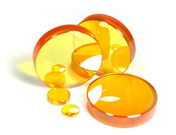
The first optical materials that could be diamond turned commercially were infrared materials like germanium and zinc selenide, as well as metal mirrors like copper and aluminum. Today, multi-axis grinding and polishing machines have expanded the list of materials that can be used for aspheric lens applications.

Cost has also been a factor in users adopting aspheric lenses. Until the last decade or so, aspheric lenses were extremely expensive compared to the simpler spherical designs. Only the most demanding applications could afford to use aspheres. And in many cases users resorted to multi-lens systems to achieve their performance goals. Today, aspheric lenses are more affordable and widely used in many industries.

Aspheric Math

It is possible to define a surface with a general polynomial such as:

Restricting our designs to rotationally symmetric optics, we can remove all the odd coefficients since they will produce a tilted or offset surface. And we can remove the zero term since this is just an offset to the curve - also of no use in our application.

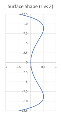
Using this equation and suitable terms for the A_i coefficients we can obtain some unusual surfaces like Figure 7.

However, Equation 6 does not allow us to make full use of conic sections in our designs. It is possible to add the higher order polynomial terms to Equation 4 to get what many optics companies refer to as the "general asphere equation."

The advantage that Equation 7 provides is that the second order term is a function of the base radius of curvature (R) of the surface. This is a benefit because the base radius is used in the paraxial calculations for the lens, most importantly in the calculation of the focal length.

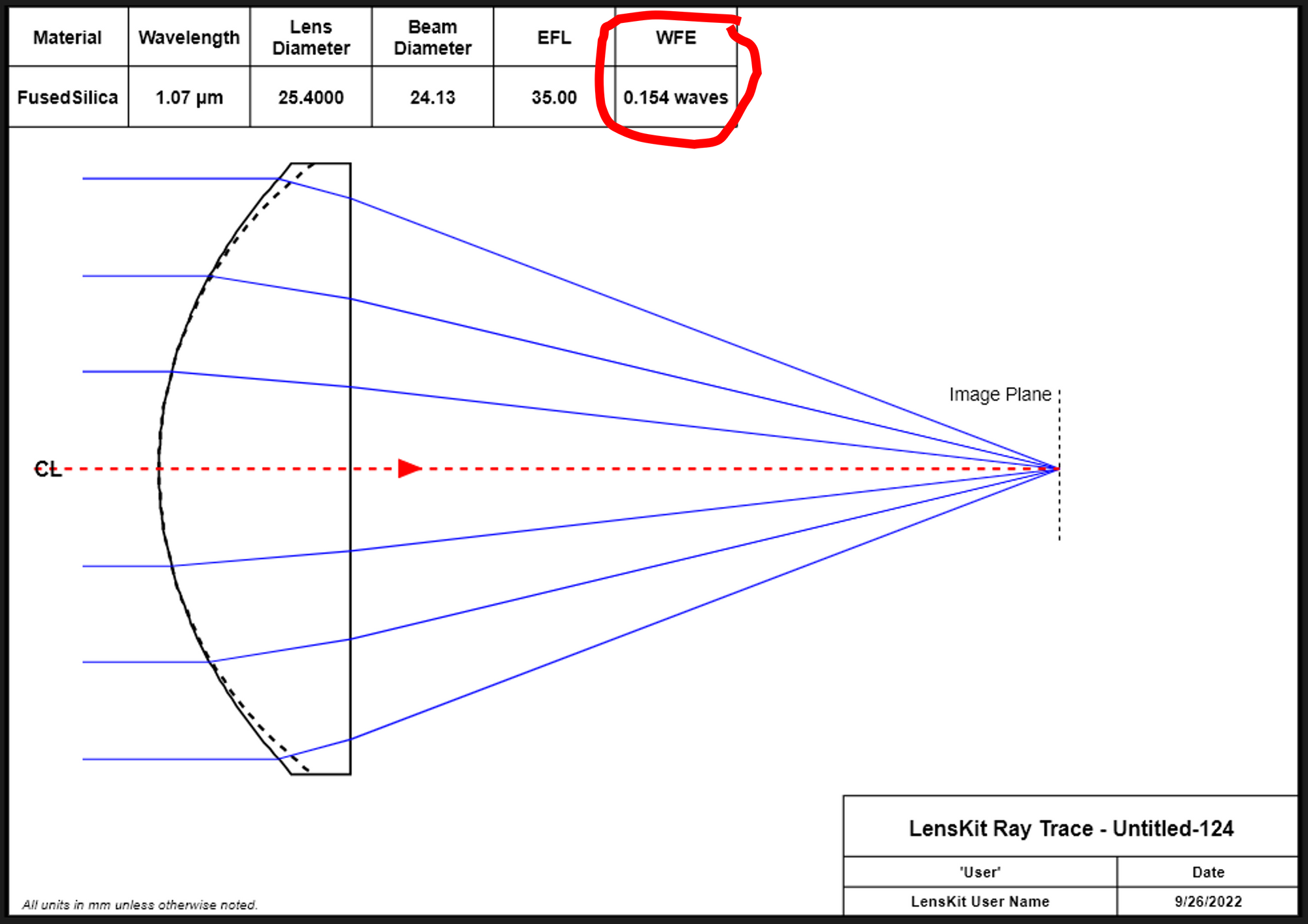
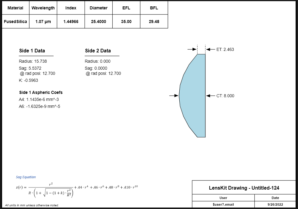
Once again optimizing the lens from Figure 1 using the conic constant, k, and the aspheric coefficients, A₄ and A₆, we can get an improved design as shown in Figure 8. Note that the WFE is reduced to 0.164 waves. Figure 9 shows an engineering note for this optimized asphere.

The mathematics for aspheres is a little bit more complex. One would not want to manually tweak the aspheric coefficients or the conic constant to improve the performance of a lens. It is possible, but extremely tedious. Fortunately lens design programs, like lenskit.app, have optimization routines that make this type of optimization quick and painless. Figure 10 shows a lens slowly being optimized to produce an almost perfect focus.

Final Notes About Aspheres

Here are a couple of thoughts about designing aspheres.

One is that the design should use the lowest number of conic/aspheric terms. It is sometimes tempting to just allow all the variables (conic plus all aspheric terms) to vary. It is a quick way to drive spherical aberration towards zero. But this adds unnecessary complexity to the design. Designing with the fewest number of terms will ensure less chance of errors when the design goes into production.

Two, in positive focal length focusing lenses, it is best to make side 1 the aspheric side. Probably a more general way to say this is that the side of the lens with the shortest radius is the one to aspherize. This probably isn't as important as the first rule, and there are cases where this may be undesirable, but it is a rule that will work in most cases.

Next up: Snell's Law and Tracing Rays